
Twelve months later, central banks had raised rates at the fastest pace in four decades. The exit window had closed. Aurora’s planned sale of two portfolio companies was postponed “until markets normalise”. Distributions were not 18% below plan. They were close to zero.
At the same time, capital calls kept coming. The subscription line had to be extended at a much higher margin. Two portfolio companies on floating-rate debt came close to their interest cover covenants. The fund’s limited partners (“LPs”) were fighting a denominator effect of their own and asked, politely but firmly, about the timing of distributions.
The CFaR model was not wrong in a technical sense. It did exactly what it was built to do. It measured variability around a plan, calibrated on a calm history. What it could not do was imagine a world in which the plan itself stopped being valid.
Fund Aurora is a composite. The pattern is not.
In April 2019 I wrote that CFaR does not work as well as it should for Private Equity Funds (“PEF”). My argument had three steps:
Seven years later, I still stand by all three points. Fund Aurora is exactly the case of point 2: a model calibrated on a benign decade produced a benign number.
Regulators have gone the same way. ESMA’s guidelines on liquidity stress testing (“LST”) for UCITS and AIFs, applicable since September 2020, are built on scenarios, reverse stress tests and the interaction of assets and liabilities. They do not ask for a single statistical figure.
A risk manager who never corrects his own models should not be trusted with anyone else’s. So here are three things I would write differently.
First: VaR is not a “maximum loss”. It is a quantile, the loss that is not exceeded with a given confidence. Beyond that point, losses can be much larger, which is why Expected Shortfall (“ES”) has replaced VaR in the Basel market risk framework. And historical simulation is not automatically the most conservative method. With a calm lookback window, it can understate risk badly. Fund Aurora’s history was exactly such a window.
Second: the data problem depends on whose cash flows you look at. For a single portfolio company, the data is too thin. At fund level, however, capital calls and distributions of thousands of funds can be pooled from commercial databases. This is the basis of the Takahashi–Alexander model (the “Yale model”, 2002) and the stochastic models of Buchner, Kaserer and Wagner. For an LP planning liquidity across a programme of funds, CFaR-type tools work reasonably well. For a General Partner (“GP”) looking at twelve companies, they do not.
Third: it is not “expert judgement or models”. In 2019 I made it sound like a choice. It is not. Pure scenarios have a weakness: without probabilities, you cannot aggregate them, compare them or allocate capital against them. Pure models have the weakness described above. The strongest approach uses expert judgement to design the scenarios and quantitative tools to discipline them. The rest of this article shows how.
In 2019 the discussion was academic. Money was free, exits were easy and distributions flowed. Since then, four things have made cash flow risk in Private Equity very real.
Thus, the question has moved on. It is no longer whether CFaR works for a PEF. It is what works instead when both the asset side and the financing side are under stress at the same time.
In 2019 I announced an article on “Quantitative Market and Default Risk Management for Private Equity Funds”. Here it is, in compact form. The idea is simple: do not model the fund’s cash flows as one black box. Split the risk into three layers, measure each with the data that actually exists, and connect them to the fund’s own thresholds.
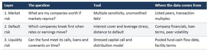
Layer 1 – Market risk: borrow the data from the listed world
A portfolio company has no daily price, but its listed peers do. Each company can be mapped to a peer group and a valuation multiple, typically EV/EBITDA. The sensitivity of the fund’s NAV to a change in that multiple then follows directly.
Two points are often missed. First, reported NAVs are smoothed, because appraisals move slowly. The volatility you see in the reports understates the real one. Statistical unsmoothing (for example Getmansky, Lo and Makarov, 2004) corrects for this. Second, equity is leveraged. If net debt is half of the enterprise value, a 10% fall in enterprise value is a 20% fall in equity value:

Layer 2 – Default risk: the covenant, not the percentile
For each company, the key question is: how far is it from breaking its interest cover or leverage covenant? Interest cover tells you how many times the company’s earnings cover its annual interest bill:

Take a company with net debt of 5.5x EBITDA and an all-in interest rate of 5%. Then raise the rate to 9%, as happened to many floating-rate borrowers in 2023. Finally, add a 15% drop in EBITDA:

Many facility agreements sit right around that last level.
For a more formal measure, a structural (Merton-type) model gives a distance to default, using asset volatility derived from listed peers. But be careful with correlation. With twelve companies, there is no law of large numbers. One common factor, rates or a sector downturn, can hit three companies at once. Concentration must be modelled explicitly, not averaged away.
Layer 3 – Liquidity risk: here the statistics do work
This is where I correct my 2019 view the most. Capital calls and distributions at fund level can be modelled with Takahashi–Alexander or stochastic models calibrated on thousands of funds. Use them, and then stress them. Replace the historical distribution rate with the recent one (6% instead of 14% of AUM), keep capital calls unchanged, and test the result against the subscription line, the loan-to-value covenant of any NAV facility and the LPs’ own liquidity needs.
Let us return to Fund Aurora with simplified numbers. The fund has invested €400 million in twelve companies. It has distributed €100 million and holds a NAV of €600 million. On plan, it will return 1.75x. The minimum the fund must deliver, to its LPs and under its NAV facility, is 1.5x. The portfolio is valued at an average of 11x EBITDA, with net debt at half of enterprise value.
Step 1 – The reverse stress test
Instead of asking “how bad can it get at 95%?”, we ask the opposite question: “what has to happen for us to miss 1.5x?”
First, two terms that Private Equity professionals use every day. Companies are usually valued at a multiple of their annual operating earnings (EBITDA). A company with €10 million of EBITDA, valued at 11x, is worth €110 million. A turn is simply one unit of that multiple. If buyers are only willing to pay 10x instead of 11x, the multiple has fallen by “one turn”, and the same company is now worth €100 million. Nothing changed in the business. Only the price the market is willing to pay for it changed.
Now the calculation, step by step:

Why the companies only have to lose about 8%. The fund does not own the whole company. It owns the equity. Each company is financed half with the fund’s money and half with bank debt. When a company is sold, the bank is repaid first and in full. The fund receives what is left. So every loss in company value falls on the fund’s equity alone.
Take one company worth €110 million, financed with €55 million of debt and €55 million of equity. Its value falls by about 8%, to about €101 million. The bank still gets its €55 million back. The fund’s equity drops from €55 million to about €46 million, a fall of about 17%. An 8% fall in company value becomes a 17% fall for the fund. This is leverage, and it works in both directions.

Translated into multiples. An 8% fall from 11x is 10.1x. In plain words: if buyers pay 10.1x instead of 11x EBITDA for Aurora’s companies, the fund misses its 1.5x. That is less than one turn.

This single sentence is more useful for a board than any percentile. Everyone in the room can judge whether buyers might pay one turn less. When rates rose in 2022, valuation multiples dropped by that much or more in many sectors within months.
Step 2 – Scenarios with probabilities
Now expert judgement does its proper job. It designs the scenarios and assigns probabilities. The model does the arithmetic.
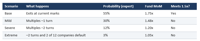
The probability-weighted MoM is 1.58x. On average, the fund meets its threshold. But the probability of missing it is 45%. An average hides exactly the information the board needs.


Step 3 – Add time
The MoM is not the only victim. If the exits in the base case are delayed by one year, a 1.75x over five years (about 11.8% IRR) becomes 1.75x over six years (about 9.8% IRR). No value is lost, yet the fund can fall below an 8–10% hurdle and the carried interest waterfall changes. Time is a risk factor of its own, and in 2023–2025 it was the main one.

Assumptions: single-period simplification, net debt unchanged across scenarios, defaults at 100% equity loss. Real models add cash flow timing, fees and the waterfall.
A practical toolkit for CROs, conducting officers and boards
If I had to set up the risk framework of a PEF again tomorrow, I would do seven things:
Imagine Fund Aurora’s board in November 2021 with a different page 14. It does not say “CFaR at 95%: –18%”. It says, in plain words: “If buyers pay one turn less for our companies (10x instead of 11x EBITDA), we miss our 1.5x. We see a 45% chance of that. Two companies breach their bank covenants if interest rates rise by 4 percentage points. Our NAV loan covenant is hit if distributions stay below 8% of NAV for two years.”
That board would have asked different questions. It might have fixed the rates on two loans, sold one company earlier or negotiated more headroom on the facility. None of this requires a perfect model. It requires the right question.
That was my point in 2019, and it is still my point today: in Private Equity, risk management is not about predicting the number. It is about knowing how far you are from the edge, and what pushes you over it.
I would be glad to hear how you approach this in your fund. Which threshold do you watch most closely, and which tool has actually helped you?
Sources
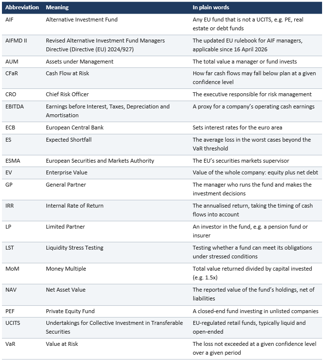
Glossary of abbreviations
From newsletter sign-up to a personal demo – we look forward to hearing from you!